Ecosystems are under threat worldwide and habitats are becoming more fragmented. Meanwhile, organisms interact with each other and the environment across long distances and, as the climate changes, will need to move to new sites as their old ones become unsuitable. Sites across a wide area can be thought of as an “ecological network” and to be really effective these networks need to be bigger, better and more joined up. This may require creation of new habitat or restoration of existing sites. Policy makers and nature conservation practitioners are increasingly thinking about conservation and biodiversity at large spatial scales, but continuing development leads to difficult decisions about how to prioritise habitat creation, restoration and even loss.

Condatis is a decision support tool to identify the best locations for habitat creation and restoration to enhance existing habitat networks and increase connectivity across landscapes. It achieves this through modelling very long-distance, multi-generation shifts across a fragmented landscape, which species are increasingly embarking on due to pressures created by climate change, amongst other drivers.

What does Condatis do?

· Highlights pathways that allow both dispersal and multiplication of species as they cross a landscape

· Pinpoints bottlenecks in the habitat network (where there are restricted opportunities for colonisation)

· Ranks the feasible sites for habitat creation and restoration to enhance the existing habitat network efficiently

Condatis achieves these outcomes through performing two types of analyses: flow and prioritisation.

Flow is a measure assigned to each habitat cell that gives an indication of the relative number of individuals moving through that cell that will go on to colonise the target (strictly speaking, their descendants will colonise the target). The larger the flow value of a habitat cell, the more important that cell is for connectivity between the source and the target. Flow of individuals only occurs through habitat cells (defined by the uploaded habitat raster map). An optional addition to the flow analysis is to visualise the most serious Bottlenecks, where flow is being restricted because of a lack of habitat.

Prioritisation is a method for prioritising patches of habitat for restoration or protection, when the user has a restricted map of feasible areas. The method shows how additional habitat cells can increase the speed of species’ movement across a landscape of existing habitat and can also be used to highlight areas of an existing network that cannot afford to be lost due their contribution to connectivity. In a prioritisation analysis, habitat cells are ranked according to their contribution to the speed of species’ movement and the lowest-ranking additional cells are ‘dropped’ from the landscape. This procedure is repeated multiple times until only the most important cells remain, contributing the most to flow.

How does condatis work?

Condatis models a landscape of habitats as if it were an electrical circuit. A circuit board consists of a number of wires joining up resistors in combinations. When a voltage is applied to the board at one end, the current will pass through the board to the other end but the amount of current passing through each wire will vary according to the resistances it meets through each pathway. Condatis considers a landscape as analogous to a circuit board (Fig. 1), with a source population of species being considered the voltage, the links between habitat useable by these species being the resistors, and the flow of species colonising the available habitat across those links being considered the current. A full description of the underlying scientific method can be found in Hodgson et al. (2012) and Hodgson et al. (2016).

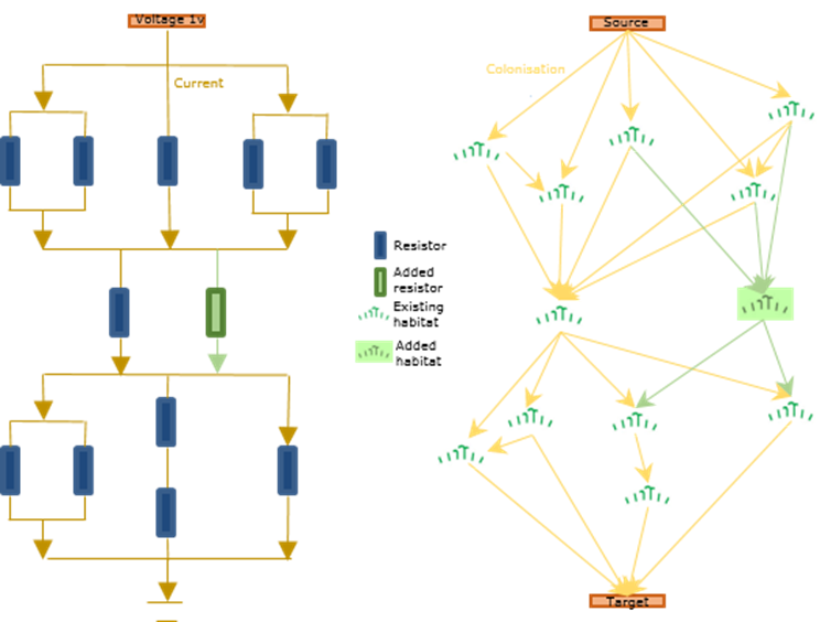
Electrical circuit on the left with resistors in blue, and stylised map with existing habitat in brown. Green represents adding a resistor or additional habitat to each to increase the number of pathways available.

Fig. 1 Electrical circuit on the left and comparable stylised habitat map on the right. Green represents adding a resistor or additional habitat to each to increase the number of pathways available and therefore improve the flow.

What does Condatis measure?

The key output of Condatis is a measure of flow (Fig. 2).

What is flow2

Fig. 2 An illustration of flow and some of the main variables modelled in a Condatis analysis.

Each habitat cell is assumed to be linked with every other habitat cell; the strength of each of these links is dependent on the time it would take for the population of one cell to send colonists to populate the other cell. The time taken is considered analogous to resistance in the Condatis model. By selecting a dispersal distance (the average dispersal distance per generation) and the reproductive rate of a species (either known or representative), Condatis will calculate the overall flow from source to target and the portion of this flow travelling through each individual habitat cell. This is plotted on a map, colour coded to highlight the areas of most concentrated flow. Condatis also calculates the time it would take for the species to colonise the target (in number of generations) and the overall flow speed which is a measure of the connectivity of the landscape and is directly comparable across different scenarios and habitats.

Is this the right software for me?

Condatis is a highly flexible and very powerful tool designed for landscape scale studies of connectivity over successive generations of species. It works particularly well for habitats that are well-defined and patchy. If you are looking for a quick and easy to use application to look at directional connectivity over a landscape, pick out the most effective sites for habitat creation or restoration, test climate change resilience or run a number of directly comparable colonisation scenarios then we would recommend trying Condatis. Only if the area of interest is very small (roughly the distance required to colonise the target within one generation of a given species) is Condatis unlikely to produce results that will be meaningful. The decision tree below (Fig. 1) can be used to further assess whether a Condatis analysis, and which type, is appropriate for your connectivity questions.

I. Considerations before using Condatis

Before using Condatis, the decision tree below (Fig. 3) will help you to identify which type of analysis is most appropriate for the connectivity questions you have.

Fig. 3 Decision tree to work through before you perform a Condatis analysis. Data types and options required for performing a Condatis analysis are shown in the pale blue boxes; * indicates raster files.

Once you have identified if Condatis is an appropriate tool for you to use, and which form of analysis to perform, i.e. flow only or prioritisation, consider the following key questions before you start your analysis:

(i) What kind of species are you interested in?

(ii) Why do your species need to move between the focal source(s) and target(s)?

(iii) What constitutes habitat for those species within the landscape, e.g. native forest?

(iv) Are you performing a bottleneck analysis, i.e would you like to evaluate where flow is most seriously restricted? [No = perform Flow only; Yes = analyse Bottlenecks

(v) Are you performing a prioritisation exercise, i.e. would you like to prioritise extra protection of existing habitat or restoration of degraded habitat? [No = perform Flow only; Yes = perform Prioritisation]

(vi) If yes to Prioritisation, how will you classify the landscape into baseline habitat (that you assume will not change in future) and the prioritisation layer (which may or may not be habitat in future)?

(vii) Who will be interested in the results, i.e. target audience? Why?

Considering the answers to these questions will help to make your Condatis analysis most useful for understanding future movement patterns of wildlife and guiding more sustainable land management decisions on the ground. For an example of answers to these questions for a specific case study, see the Condatis Training Exercise (Specifically Condatis_TraningWorksheet.pdf).

2. Running an analysis in Condatis

I. Getting started

Condatis web version 1.2 can be accessed here. In order to use Condatis, you will need a laptop/desktop computer with access to the internet. Condatis will work on any browser, and requires you to create a personal account before you can access the tool. If you have any difficulties registering for an account, please email contact@condatis.org.uk. For more information on this decision support tool, its origin and the Condatis projects currently underway, please have a look at our website. If you do not have your own data to run, you can access some pre-prepared training data on the Training resources page of the website, which forms the case studies used below to illustrate the tool.

II. Input files and variables

The data layers/values that are required for running a Condatis analysis are shown below, along with a brief description of how to create each input.

Data layer/PARAMETER	Explanation
Reproductive Rate (r)	Derived from ground data/expert knowledge, or based on a general rate to replicate slow, medium and fast reproducers. As a rule of thumb 10 or less will show movement of low fecundity species, 100 or more high fecundity species. This is effectively the number of emigrants leaving 1km² of suitable habitat every generation. As the speed of colonisation (and therefore time taken) is simply multiplied by R, the speed of colonisation for any rate of reproduction can be easily calculated once the initial scenario has been run; measured in individuals per km².
Dispersal Distance	Average dispersal distance for the species of interest, as distance from where parent is born to where offspring are born. Derived from ground data/expert knowledge; measured in km
COMPUTE BOTTLENECKS	Tick the checkbox if you wish to compute bottlenecks in your flow.
Number of Bottlenecks	Here you can provide the number of the most severe bottleneck links to display in the results and generated shape file. Attempting to display too many bottlenecks can create a confusing picture. In any case the bottleneck csv file within the results package contains the top 1000 bottlenecks regardless of the number specified for display.
Habitat	Raster which must be a geographical .tif file, where cells have a value between 0 and 1 , according to the quantity/quality of habitat within each cell: 0 being empty of habitat, 1 being completely full. Alternatively, it can now be in the form of a categorized .tif file (see CATEGORIZED HABITAT below
CATEGORIZED HABITAT	You can now also present what we are calling categorised habitat tif files. Different types of habitats within your habitat file are denoted by distinct integers. (For example 1 could signify heathland, 2 forest and 3 marsh etc.) You will be asked to input habitat quality for each habitat category when presented with the preview report.
Auto Source & Target	Tick the checkbox if you wish to automatically generate a source and target layer. Once ticked a choice of 4 directions are made available. North to South, West to East, South to North and East to West, corresponding to source to target directions. The generated TIF file is made available in the results package.
Source and Target	If supplying your own Source and Target layer than it must be a raster which must be a geographical .tif file with the same coordinate system as the Habitat file; source grid cells (pixels) are given a value of ‘1’ and target cells ‘2’. Where cells overlap the habitat cells then the conflicting habitat cells will be automatically removed.

*For Prioritisation* analysis only:**
Prioritisation	Raster which must be a geographical .tif file with the same coordinate system as the Habitat file, which can represent habitat that either: (a) does not currently exist, but where restoration is possible, or (b) does exist but is currently unprotected and therefore may be a priority for conservation. In case (b), the unprotected habitat will be automatically subtracted from the habitat layer before processing.
Stages	Choose which number of stages is appropriate given the desired specificity of results (better with more steps) and time available for analysis (slower with more steps).
Stage Type	The two options are: (i) Number based (equal number of cells dropped in each stage), or (ii) Flow based (equal proportion of flow dropped in each stage). The number based output may be simpler, for ranking the landscape into broad bands, but the flow based output gives more detail in the high-flow areas, which we think may be more useful when you can only afford to protect/restore a very small proportion of the additional habitat.

Before you are ready to perform an analysis in Condatis, you need to create the input raster files for the analysis: source/target and habitat layers, and prioritisation layer, if you are performing prioritisation. These raster files can be created in a GIS programme, R or by using another programming software. It is advisable to view your input layers in a GIS viewer after creating them, to ensure:

· The spatial resolution of cells/pixels and map projection are the same in all raster files;

· The spatial extent of all raster files are exactly the same, i.e. have the same bounding box;

· All raster files are in geoTIFF format, i.e. labelled .tif.

· The source/target layer contains only 1s and 2s; and,

· Habitat coverage is measured in proportion or percent (unless you are using a categorised habitat file).

Further guidance on how to create the appropriate input layers is provided in our collection of raster demonstrations.

III. Completing a ‘job’

1. Open Condatis webapp & register or sign in.

2. Select create new job.

3. Give your job a meaningful title.

4. Set the reproductive rate for your species of interest.

5. Set the dispersal distance for your species of interest.

6. Upload your habitat layer. Condatis requires a landscape pattern to work with. This will usually be made with some kind of GIS software such as ArcGIS, Mapinfo or QGIS.

7. Define a source and target. Condatis calculates the flow between habitat patches defined as the source and patches defined as the target. These can be either generated automatically or loaded as GIS layers.

8. Select bottlenecks if required. Select how many bottlenecks you wish to display in the results .html. The bottlenecks .csv file will contain the top 1000 bottlenecks, regardless of what you select to display.

9. Select prioritisation if required. An option will appear to upload your prioritisation layer. Decide how many stages you require for the dropping procedure and whether those stages should be number based or flow based.

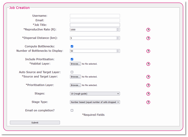
10.Click Submit.

11.You will be asked to wait whilst the server does some checks on the validity of your submitted data and job.

12.Once the checks have been carried out, it should only take a few minutes you will be presented with the preview screen. Assuming no problems have been found and in the case of a standard non-categorised habitat layer you will be asked to confirm submission.

Graphical user interface, text

Description automatically generated

Should your habitat layer be categorised you will be asked to enter the habitat qualities (between 0 and 1) you would assign to each habitat category type.

An extra feature is the button Add Species. This allows the user to use the same categorised habitat file for different species, as each habitat category may be better for one species than another. Each species can have its own dispersal distance.

Once the habitat qualities have been assigned the data can be submitted in the usual way.

If you have provided more than one set of category habitat quality values (that is for more than one ‘species’) then each set will be submitted as a separate job.

Graphical user interface, text, application

Description automatically generated

13.Your position in the Queue will be shown.

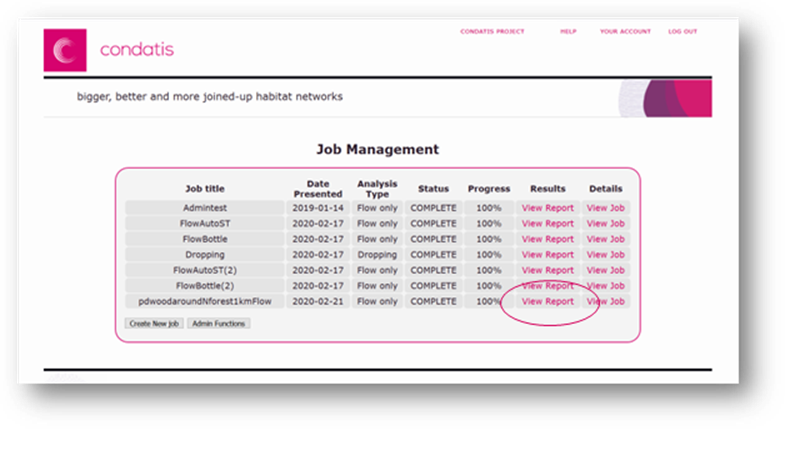
IV. Obtaining results

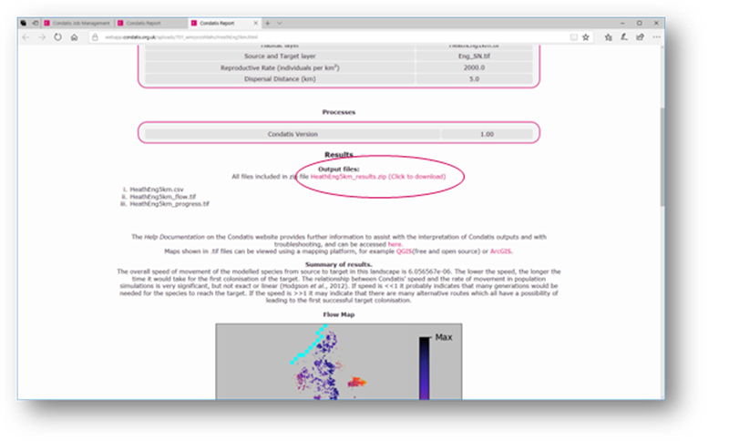
When your job has finished running, open the results html page by clicking “View Report”.

And download the zip file containing your outputs

Further guidance on running an analysis in Condatis can be found in the Condatis Training Exercise

V. Re-running a job

If you would like to run the same job again, but with slightly modified parameters, you can do this by clicking on the “Create Related” tab in the “View Job” tab of a previously completed job. Input files and parameters will be exactly the same as the viewed job, with the only difference being the (2) suffix on the job title to ease navigation between jobs. The job title and all other components can be modified as required.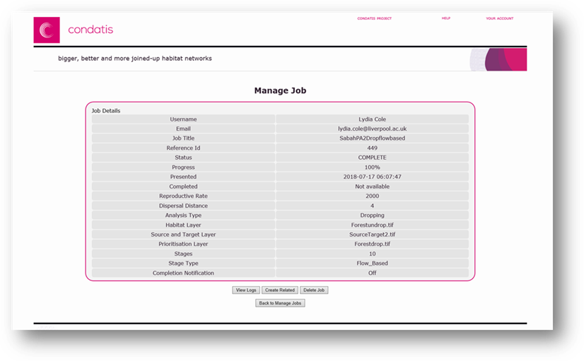

If you need to delete a job altogether, use the “Delete Job” tab on the same Manage Job page. However, if the job failed, please check with contact@condatis.org.uk before you delete it so that the development team can interrogate the job to find out what might have caused the failure before the evidence is lost! If you have run more than 16 jobs, only the first 16 will be shown on the Job Management page to reduce the requirement for scrolling; if you would like to see an earlier job or count your total number of submissions for example, click the “View All” tab at the bottom of the page.

3. Interpreting results

I. Output files

The output/results files from a Condatis analysis are shown below. Figure legends in the results .html file contain descriptions of each output.

Results file	File type
FLOW ONLY
Flow	.csv
Overall speed	value in .html
Flow	.tif
Progress	.tif
Bottlenecks (optional)	.csv
Bottlenecks (optional)	shapefile

PRIORITISATION (in addition to FLOW outputs above)
Drop	.csv
Change in speed of movement	value in .html
Trajectory of dropping	Fig. in .html
Dropping Rank	.tif
Start Flow	.tif
End Flow	.tif
Step Dropping Summary	.csv

II. Interpreting outputs

Basic guidance on interpretation is given in the figure legends of the .html file. For a more detailed explanation, see the Condatis Training Exercise presentation.

Flow through each cell. This map highlights where the focal species is most likely to colonise on its way between the source and the target. Cells with high flow are priorities for conservation because, if they were lost, the overall speed is likely to suffer. The flow is sometimes very "concentrated" in one major route through the landscape, and sometimes more diffuse. Bear in mind that diffuse flow is not a bad thing - in fact it means that there are many alternative routes the species could take.

Progress. This map shows a gradient where habitat patches near to the source will have progress values close to 1 and patches near to the target will have progress values close to 0. This indicates the order in which cells are likely to be colonised through time. For example, out of the overall time taken to reach the target, half will be taken getting to wherever the progress shows 0.5, and the other half of the time will be taken crossing the rest of the landscape. If the landscape is very blocky (big blocks of habitat with big gaps), the cells within one block will be close together in progress (because the species will spread through there very quickly), and between blocks there will appear to be gaps in progress (because there will tend to be a long wait before the next block gets colonised).

Bottlenecks. This map helps to identify the places where new habitat would be most beneficial to colonisation speed. In our model, every cell has a link (however weak) to every other cell. By looking at the properties of these links we can find those that straddle bottlenecks. A place is a bottleneck if it has high resistance and yet forms part of one of the best available routes through the landscape. If habitat were added on or around the lines representing these bottleneck links, then the whole route would have significantly higher flow. Therefore, the map of the top bottleneck links gives suggestions of where you would ideally add habitat, if you could only make one change to the network. Since every cell in the landscape is connected to every other cell in the landscape there are a large number of links. It would be meaningless if all the links were plotted. Instead, the software plots only the links that have the greatest power relative to the cumulative power. The number of links plotted is controlled by the value set when creating your job.

Dropping Rank Map. This map shows the cells from the new layer ranked in terms of their contribution to flow. Lower-ranking cells were dropped earliest because they carried relatively little flow. Higher ranking cells were retained longer, and this implies that they are of higher priority.

Trajectory of dropping. The speed, (inversely related to the time taken to cross from source to target), is plotted against the stage of dropping. Speed is expected to get slower when habitat is lost from the landscape, but notice how severely speed is lost at different stages.

Glossary

Term	Description
Bottleneck	A gap between habitat patches that lie on a major path of flow. Adding new habitat in these gaps will improve the flow along the associated path, improving overall flow between the source and target.
Cell	The square spatial units from which a raster layer is comprised.
Conductance	See Speed
Connectivity	The ecological proximity between two habitats, i.e. how well connected two habitats are relative to the species travelling between them. How connected two patches of habitat are for an individual depends on the distance between them, the characteristics of the intervening landscape and the ecological characteristics of the individual, e.g. dispersal distance and habitat preference.
Dispersal distance	The average distance one individual can travel in their lifetime; derived from ground data/expert knowledge per species; measured in km.
Dropping	Dropping is a method for prioritising patches of habitat for restoration or protection, when the user has a restricted map of feasible areas. The method shows how additional habitat cells can increase the speed of species’ movement across a landscape of existing habitat and can also be used to highlight areas of an existing network that cannot afford to be lost due their contribution to connectivity. In a prioritisation analysis, habitat cells are ranked according to their contribution to the speed of species’ movement and the lowest-ranking additional cells are ‘dropped’ from the landscape. This procedure is repeated multiple times until only the most important cells remain, contributing the most to flow.
Extent	The geographical range of the landscape of interest, defined by coordinates. For Condatis analyses, the extent of an input raster file must be defined in meters.
Flow	Flow is a measure assigned to each habitat cell that gives an indication of the relative number of individuals moving through that cell that will go on to colonise the target (strictly speaking, their descendants will colonise the target). The larger the flow value of a habitat cell, the more important that cell is for connectivity between the source and the target. Flow of individuals only occurs through habitat cells, defined by the uploaded habitat map.
Habitat	Habitat constitutes a land cover/ecosystem type in which a species is able to survive and breed, thus it contains all of the resources required for the species of interest to obtain shelter, adequate nutrition and opportunities for reproduction. The Habitat layer forms the primary raster file to which the other geospatial layers are matched in a Condatis analysis. The required geospatial input layers, prepared as rasters in .tif format, with the same coordinate system and measured in units of metres, are: (i) Habitat Layer; (ii) Source and Target Layer, and (iii) Prioritisation Layer. Each layer consists of a grid of habitat cells (see below); what constitutes “habitat” is dependent on the taxa chosen for the analysis, e.g. within the same landscape the grid of habitat cells for a termite and a chimpanzee may have quite a different configuration.
Habitat cell	A habitat cell is a grid square or pixel within the raster input layers. The value given to each cell is equivalent to the coverage of habitat within that cell (between 0-1 or 0-100%). Cells with no habitat may be coded as 0 or ‘nodata’. The number of habitat cells in the raster affects the time it takes for the Condatis analysis to run: for example, analyses for habitats of up to approximately 20,000 cells can be quickly calculated, whereas if there are many more than 50,000 cells in a flow analysis it will slow down significantly, or may prove computationally impossible for a prioritisation analysis.
Habitat creation	Any process that creates functioning, breeding habitat where none exists currently.
Job	An analysis performed in Condatis, i.e. a flow or prioritisation analysis performed in the online version of the tool, defined by a specific set of input files and variables.
Landscape	The geographical area over which a Condatis analysis is performed, defined by the extent of the Habitat layer.
Network	Condatis is a network model, and analyses the strength of connections across this network. The network represents in a simplified way how the species of interest can reach any habitat cell from any other.
Pixel	See ‘cell’
Prioritisation layer	This layer defines either currently unprotected habitat to assess for conservation or non-habitat to assess for restoration. Each cell represents habitat that could be protected/restored to extend the current network of habitat through which the chosen taxa could move. The Prioritisation layer is used in the prioritisation analysis, to explore which additional habitat could contribute most to increasing flow across the landscape and therefore be important to prioritise in conservation/restoration interventions. See also ‘Dropping’.
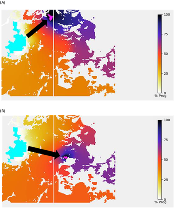
Progress	Progress provides an indicator of the relative time spent by the species of interest moving across different parts of the landscape from the source to the target habitat. An even distribution of colour indicates that movement across the landscape is relatively uniform, i.e. it takes a similar amount of time to move through each habitat cell between the source and target (illustrated by Fig. A); whereas the dominance of one colour suggests rapid movement through that section of landscape with the bunched colours representing a bottleneck or other features that restrict movement (illustrated by Fig. B), where 50% of the total Progress of the source-to-target movement is not achieved until approximately 75% of the linear distance has been crossed). Fig. A & B Two example Progress reports from the Condatis web version. The source is shown in blue, the target in pink and the main channel of movement is delineated by the black arrow; lighter colours represent proximity of the species of interest to the source habitat and darker colours proximity to the target, with values reported as a percentage of the total movement across the landscape.
Range shift	The directional, long-term movement of the habitat of a population, often driven by climatic changes that cause the previous geographical range of a population no longer ecologically suitable.
Raster	A common format of geographical data, see https://desktop.arcgis.com/en/arcmap/latest/manage-data/raster-and-images/what-is-raster-data.htm
Reproductive Rate (R)	This represents the average number of individuals produced per generation per km² of habitat for the species of interest. It is derived from ground data/expert knowledge.
Resistance	The inverse of conductance, analogous to the time taken for colonisation to occur (from one cell to another, or from source to target)
Resolution	The size of the cells within a raster layer.
Restoration	An activity performed by humans with the goal of rehabilitating degraded habitat to a former quality/quantity.
Source	The source is chosen by the user and represents the start-point of population movement for the modelled species moving to the desired target. Sources are patches of habitat that were of suitable biophysical composition and size to accommodate the modelled species/taxonomic group now or in the past. The assumption is that movement between source and target will be necessary for some reason, e.g. as the source becomes climatically unsuitable, too hot and/or too dry.
Speed	This is a measure of overall or total flow, i.e. successful movement of a species/taxonomic group from the source to the target. The faster the speed, the shorter the time taken to reach the target, measured in units analogous to generations of individuals. The speed reflects the time taken (in relative units) for the fastest individual to move between any source cell and any target cell (not necessarily colonisation of the whole target area or movement of the whole population). If the landscape configuration changes and/or the species being modelled changes, the speed will change. For example, if a species has a shorter dispersal distance, or produces fewer individuals per km² per generation, all movement through the landscape will be slower. Landscape configuration can also have a large impact on speed (see Hodgson et al., 2016 for more information on this). Speed is a relative measure that can be compared across scenarios computed by Condatis.
Stages	The user only needs to consider this parameter in a prioritisation analysis. Habitat cells within the Restoration Opportunity Layer are removed using the chosen number of stages, each one corresponding to a stage of ‘dropping’. If more stages are included, the analysis takes longer because it is repeated for each stage; however, the user is able to differentiate more between habitat cells in terms of their contribution to overall speed, rather than large ‘chunks’ of cells all having the same contribution. The options for the number of stages to perform are: the maximum of one cell dropped at a time, 1000 stages, 100, 50 and 10 stages. The recommended number of stages is 100, as a compromise between spatial resolution and time taken for the analysis to run. The options provided for “Stage Type” in the web version of Condatis are: (i) Number based (equal number of cells dropped in each stage), or (ii) Flow based (equal proportion of flow dropped in each stage). The number based output may be simpler, for ranking the landscape into broad bands, but the flow based output gives more detail in the high-flow areas, which we think may be more useful when you can only afford to protect/restore a very small proportion of the additional habitat.
Target	The target is chosen by the user and represents the desired end-point of population movement for the modelled species moving from the source. Targets are patches of habitat of suitable biophysical composition, size, and in some cases predicted future climate, for the modelled species/taxonomic group. When considering the future movement of species under climate change (one of the primary applications of Condatis), the target could be an area which will have the same climatic conditions in the future that are found currently in the source, according to available climate models. The assumption is that movement between source and target will be necessary as the source becomes climatically unsuitable, e.g. too hot and/or too dry.
Time	A relative measure of time, reported in units analogous to generations of individuals.
Voltage	See Progress

FEEDback & questions

If you have any questions that have not been answered in this help document, or feedback to share, please email contact@condatis.org.uk.

The text of this report is copyright Condatis team 2018. The report is intended for the use of the registered user and his or her immediate colleagues. If you wish to disseminate the report or any extract of the text more widely, please seek written permission by emailing contact@condatis.org.uk.

How to cite Condatis

For preferred citation formats, please refer to our website.
Most recent publication of the underlying scientific method: Hodgson, J. A., Wallis, D. W., Krishna, R., & Cornell, S. J. (2016). How to manipulate landscapes to improve the potential for range expansion. Methods in Ecology and Evolution, 7(12), 1558-1566. Doi:10.1111/2041-210X.12614.